Using BadElf GPS with IOs device

Introduction:

GPS's are very useful devices that are getting more and more useful with advancing technology.  The software that supports GPS units is ever advancing and creating new opportunities for GPS application.  This lab goes through the possible applications of the BadElf GPS and its use with an IOS device.

Methods:

The BadElf GPS is a hand held GPS unit that can be linked to an Apple IOS device via bluetooth.  They make a range of units from survey grade to a version that plugs into the lightning port of an apple device to get about 10ft gps accuracy.

BadElf has a free app that supports a variety of features for their gps units.  For the purposes of this lab, the tracklog feature was demonstrated.  Once paired with their devices, the class headed outside.  Once outside, the bottom button was held down and the tracklog mode was activated.  This enabled the gps unit to start recording data.  The class was then instructed to walk around campus.  After 15-20 minutes the class regrouped and downloaded the tracklogs onto the BadElf App.  This was done by going to the app and simply selecting "Download Tracklogs."  After the tracklogs were downloaded they had to be put into a format that could be put onto a computer.  The app comes with a share feature that does this for the user.  The share button allows the user to send the tracklog as a KML or a GPX with an email.  The KML can be brought into Arcmap and converted into  a layer file.  This layerfile is then exported into a feature class and can be used in the map like the one below.

This is one application that the bad elf can be used for.  There are many other application that can be used with a BadElf gps. Collector and Survey 123 are two applications developed by esri.  Collector is a data collection application that allows for people in the field to collect data onto maps that have been set up.  Survey 123 is a form based application that allows the user to make forms that create features that can be used in collector.  A BadElf gps can be used to collect more accurate data gps data for these applications.

GIS4Mobile, Theodolite, Gaia GPS, and Galileo Offline Maps, are all mapping applications that can be used with the BadElf GPS.  The gps is used to create higher accuracy for the applications.  A phone gps is not very accurate and using the BadElf gps with these applications can get the accuracy to within a foot depending on the unit.

Conclusion:

With software applications being developed everyday, the use of an external gps is getting easier to use and it is able to be used in many more situations.  For a few hundred dollars, anyone can purchase a gps unit that easily connects to a phone and is in sync with a multitude of mapping applications. This will continue to evolve and the uses of gps's with keep growing!

Navigation Map

Introduction:

Being able to navigate is one of the most important skills to have.  The world is a large place and in order to get around without getting lost, a person must possess the skill to navigate! Throughout history people have been navigating from using the stars and sun to using a gps in todays day and age.  Besides just a gps or compass, a person will need a map to help assist them in navigating to a place.  This assignment is to create navigation maps for a later time to assist with groups finding their way through the woods. One map will be focused on assisting navigation with a compass and using step counts.  The other map will be focused on assisting GPS navigation.  Each map will contain specific items that make them useful in assisting in gps, or compass navigation.

Methods:

To create a map that is useful to navigating with a compass, a coordinate system based off of meter must be used.  It would be no use to have coordinates on this map because it will not help a person locate themselves.  Knowing they are "35 meters" from that creek will be useful but not "that creek is at 35.23345 degrees north."  For the first map, A grid will help the user understand distances using meters. This map was created using data provided by Professor Hupy.  First the map and data had to be put into the proper coordinate system and projection.  In this case it was wgs 84 UTM zome 15n.  This allows for the meter grid system.  Once this was done, the proper 11x17 map layout was set and the map was created.  The UTM map shows a grid in meters that will allows the person viewing the map to navigate based off landmarks and distance.


The second map created was similar to the first map except everything was projected into a local coordinate system of NAD_1983_HARN_WISCRS_EauClaire_County_Feet.  This map has a coordinate grid instead of a metered grid.  This allows for the map to have a local coordinate system.  The same procedure was used to create this map.

Litchfield Mine Survey

Introduction:
This class is a upper level geography course that teaches the basics of how to do field work.  This week's lab was a field day at a local mine designed to show the students how to do basic GPS survey and to introduce them to a variety of Unmanned Aerial System platforms and one robotic total station.  With technology advancing faster than ever, today's survey techniques are very advanced and accurate.  With the use of UAS (Unmanned Aerial Systems) a mine can be surveyed in a few hours with centimeter accuracy.  This lab was designed to show the differences between multiple GPS and UAS platforms.

Both sections of Field Methods met at the Litchfield mine on a Saturday, September 30th.  This mine is located just southwest of Eau Claire WI.

Methods:

To begin the day the class walked around as a whole and placed out Ground Control Points for later use with the drone imagery.  The GCP's were set out in a way that none of them were clustered together in one area and they were spread on a variety of surfaces.  Some on top of piles of material and some on the low ground.  To get accurate measurements of piles, GCP's were placed on top, and around the largest piles.  A GCP is just a square that is placed on the ground that is taken with a GPS.  This makes it a known point and allows the imagery to be tied down to where it is in the world accurately.  After laying down the GCP's, the class was split into groups to go take coordinated of the GCP's with a variety of GPS's.  These GPS's included:

-Iphone
-Bad Elf GPS Unit
-Trimble R2
-Septentrio Altus NR2
-Arrow GPS Markers
-Topcon HiPer


The accuracy of these GPS's are to be compared when the data is processed at a later date.  Some of these units have sub-cm accuracy and some have around 10m accuracy.  The purpose of this lab and field day is to compare what units are actually more accurate.  The following link is a link to the Bad Elf and Iphone GPS Coordinates. The other data is not yet processed.

https://universityofwieauclaire-my.sharepoint.com/personal/bealir_uwec_edu/_layouts/15/guestaccess.aspx?guestaccesstoken=W9LCwEn%2f9mv843morGhbvirEw7%2bbscnLlBTRUwJL2qI%3d&docid=2_09c2590b8e4a049eda216cf5714bb358f&rev=1

The following map is a hand drawn map of where the GCP's were located.  This is to help find the GCP's when processing the imagery.

Once the GCP's were recorded with a variety of GPS's, it was time to fly! The first UAS to fly was a DJI Phantom 3 Pro.  DJI is one of the most popular brands of drone for public and commercial use.  The Phantom series is their most popular drone.  With about a 25 minute flight time this drone is a great portable drone for taking aerial imagery.  There are a variety of flight planning apps that allows the pilot to create a grid that the drone will follow for mapping. The program has the drone take off, fly the pattern, and land.  The image overlap, flight height, speed and other settings are set during the mission planner.  This is an affordable platform ($800-$1200) that is good for basic mapping applications

Phantom 3 Pro

The second UAS to fly was a SenseFly eBee.  This a fixed wing aircraft with a foam body that requires little to no flying skill for the pilot.  The Pilot in Command creates a flight plan using the app that the UAS comes with from SenseFly.  This is where the pattern the drone is to follow is set, as well as things like height, speed, rally points, and other things the platform needs to fly.  When the mission is planned the PIC (pilot in command) shakes the drone three times and throws it.  The eBee knows its suppose to start the mission and takes off into the sky. The eBee is a high level mapping UAS platform that is capable of getting centimeter accuracy with RTK GPS capabilities.

SenseFly eBee

The next platform to fly was a DJI Matrice 600 Pro.  This is a few steps up from the DJI Phantom. It has more motors and is much larger.  Instead of just one battery like the Phantom, this platform has 6. This almost doubles the battery life.  Besides the battery life and more motors, this platform has RTK GPS capabilities making it up to cm accurate. A similar mission planning software is used for the M600 as the Phantom.  One of the biggest differences between the M600 and the Phantom is the M600 can swap sensors.  A bigger more powerful camera can be put in the M600.  Different types of cameras for different applications can be put the in M600.  This is one of the biggest benefits of this platform.  The Matrice 600 falls in the range of $3000-$6000 depending on the sensor and GPS options it comes equipped with.  Putting an upgraded sensor on it is always an option and that can range from $500 to well over $50,000 depending on the sensor.

DJI Matrice 600 Pro

Last but not least the is the C-Astral Bramor.  This is by far the most expensive UAS at $70,000.  This is a high performance fixed wing drone capable of 3 hour flights.  This is an ideal platform for mapping large areas with cm accurate data.  This is a new drone on the market that Menet Aero displayed at the mine.  It is a fiberglass bodied drone with a wing span of more than 5 feet.  Equipped with RTK GPS this platform is for high end mapping applications.  The Bramor comes with an advanced mission planning software that allows for unique mapping applications like corridor mapping.  The most intriguing thing about the Bramor is it's parachute landing.  This means that it can be used when there is not a lot of room to land. 

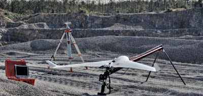
C-Astral Bramor

Conclusion:

Starting with the GPS units, the high end sub-cm accurate GPS's were very easy to use.  Once a data collection app was set up, all the user needed to do was enter a few things about the point they were taking and hit submit.  This automatically populated a feature class and stored the coordinates.  This was easier than actually writing the coordinates down for the Bad Elf and Iphone.  We will see what GPS unit was more accurate at a later date.

This day was plagued with bad luck for the Unmanned Aerial Systems.  The Phantom flight went great once some technical difficulties were solved but once the fixed wings were pulled out things started to go downhill.  The eBee flight was off to a rocky start when it suddenly did a barrel roll while flying its pattern.  The pilot got concerned and told the drone to return to home.  The drone did not want to listen and started flying very irregularly doing more barrel rolls and getting higher and higher.  Suddenly the computer started chiming, "IMU FAILURE, IMU FAILURE" and the eBee started plummeting to the ground.  This was a bad first impression of the SenseFly eBee.  The drone was located by searching for it with the M600.  The M600 performed flawlessly finding the downed drone and flying its mission. 

The last drone flight of the day was the most exciting.  The C-Astral Bramor is a large platform that performed great.  It is launched by a catapult and then fly's its mission.  It is very stable while flying even with a slight wind.  Every thing went as planned until the landing.  The Bramor started its decent as normal and once at the proper elevation came in for landing.  The class watched eagerly for the chute to open.  Panic ensued when the pilot said "Joe...the chute didn't open."  The Bramor floated over the trees and into the woods.  About 15 seconds later a loud crash could be heard in the distance.  This was a freak accident that is still being investigated.   

Distance Azimuth Survey

Goal and Background:
In today's world, technology is involved in every aspect of life.  Most people wake up from an alarm on their phone, cook breakfast on an electric stove, follow directions from their phone on the easiest way to get to work, then use a computer or tablet to assist in whatever kind of work they do.  Technology has reached a point where it is involved in pretty much everything that happens in this world.  The world of GIS is no different, changing and advancing technology is changing the way GIS is used and keeps it growing everyday.  Surveying is closely related to GIS and is also constantly changing with technology.  The old ways of pulling tape measures is in the past and the era of GPS surveying is here.  GPS technology is used in almost all surveying applications.  It is accurate and reliable.  But how reliable is it? There is always a chance that technology can fail and it is important that people know what to do if the technology is not working.  The distance azimuth surveying technique is a way of mapping distributions based around a single known point.  This would not work for mapping the location of objects but only for mapping spatial distributions.  This report will go through the method used for mapping the distribution of trees in Putnam Park on the University of Wisconsin- Eau Claire.

Methods:


The distance azimuth survey method was used to collect tree data in Putnam Park.  Groups of 3 went into the field equipped with a Bad Elf GPS, Tape Measure, Compass, and Distance Finder. (figure 1)

Figure 1

  With equipment in hand, the next step was to go out into the field to collect data.  The task was to collect data about 10 trees surrounding a certain location.  Once the location was determined, the GPS was used to get the coordinates of that spot.  These coordinates were recorded in a field notebook.  Once the spot was determined, a tree was picked and information about that tree was taken.  The distance from the recording location in meters, tree circumference, tree type, and direction from the reference point.  To get this information the tools that were provided were utilized.  To get the distance to a tree, the distance laser was used.  This device (middle right tool in figure 1) uses a laser to get distances in meters.  It is shown in action in figure 2 below.

Figure 2

To get the circumference of a tree, a simple tape measure was used.  This is an age old method that had withstood the test of time. (Figure 3)

Figure 3

The direction was collected by using a compass.  The degree and quadrant were recorded to later find the direction of the tree.  For example, the compass went from 0-90 degrees for four quadrants, this led to a calculation that needed to be done to get degrees 0-360.  Lastly, the tree type was recorded by asking our professor (who has lots of tree knowledge!) and by using best judgement.  Once all the data was collected it was normalized into a table in order to be brought into ArcMap.  The direction was converted into a format of 0-360 and each tree was given the coordinate that it was collected from.  The normalized table is shown below (Figure 4)

Figure 4

The normalized table allows the user to bring it into Arc using the coordinates of each tree.  Once the table is brought into Arc, a few tools are ran on it to get it to show the trees, reference locations, and lines that depict the direction and distance of the trees from the reference point.  The Bearing Distance to Line tool takes the coordinates, direction, and distance to create lines that depict the distance and direction from the reference point to the trees.  This tool alone does not create points for the trees or the reference location.  The Feature Vertices to Points tool can create points from the beginning or end of the line created.  This tool was ran twice to get points for the trees and points for the reference location.  The tree points were created but data about tree type and circumference was lost during the process.  To get around this a table join was done to bring in that information about the trees.  Once the join was complete the process of collecting and bringing in tree data using the distance azimuth technique was complete!

Results:

When first inputting the data, one of our locations was tens of miles away from where we actually took data.  We realized this was caused by a data entry error of one of our coordinates.  Thankfully we had a picture of the GPS when it was actually showing that location.  Once this was solved our data appeared to be in the correct location.  One thing that seems wrong is that one of our trees appears to be on the other side of the footbridge when we didn't actually take data on any trees across the footbridge from the more westerly point.   This can be seen in the map below (Figure 5)

Figure 5

Besides just being able to see the distribution of trees, the circumference data made it possible to make a map showing the circumference of the trees. (Figure 6)

Figure 6

The last map is a map showing the various tree types collected.  (Figure 7)  This map uses a unique values symbology to show the different types of trees.  There was quite a variety of trees out there!  There are only two spots where trees are grouped together.  There is a group of White Ash trees in the more westerly group and a group of Black Ash in the more easterly group.  One mistake in the data was two different spellings for white ash which resulted in two different categories for white ash. 

Figure 7

Conclusion:


The distance azimuth survey worked relatively well for this lab.  It was no the most accurate but it have some upsides.  It does not require expensive tools, can be done quick, and will work when other more advanced technology fails.  On the other hand, having an accurate GPS would allow someone to walk right up to each tree and get the location of it to within a centimeter.  This kind of GPS is expensive but would allow this job to be done much quicker and accurately.  Not just would it be more accurate the data would be exact locations and not just spatial distributions. 

Creation of a Digital Elevation Surface using critical thinking skills and improvised survey techniques

Introduction:

This lab was designed to learn how to take a sample of x,y,z data and turn that into an elevation model in Arcmap.  This was done by creating a landscape in a sandbox and taking points to be mapped at a later time.  One important aspect of this lab was deciding on what kind of sampling method we were going to use.  Since we knew the box was going to be 114x114 cm long we decided for the sake of this project a systematic sampling technique was used.  This means we took Z-data every 6 cm in the X and Y direction.  This would give the best spatial representation of what we were making.  The other sampling techniques we could have used are random sample and stratified.  Random sample is done by generation random points and taking the elevation of those points.  This is a good way to collect data but we felt that using random sample in this situation might not yield the best results.  Stratified sampling is when points are taken from certain areas in the study area and are suppose to be representative of the whole.  We decided this technique would also not yield the best results.  The objective of this lab was to use the best technique to collect the most accurate data we could.  This data will be imported into Arc and turned into a surface model.

Figure 1

Methods:

We chose to use the systematic sampling technique because we felt that taking the Z-value every 6 cm in both directions would yield the most accurate data that was representative of the whole.  Systematic and random sample did not quite fit what we wanted to do.  We built our landscape in a sandbox created by Dr. J. Hupy located in an open area directly across Roosevelt Ave from Phillips Hall at the University of Wisconsin - Eau Claire.  To create the landscape we used very advanced shaping tools called our hands.  We were sure to include a ridge, hill, depression, valley and plain.  Once our landscape was created we created a grid using thumb tacks and string.  The thumbtacks were set into the edge of the sandbox every 6 cm.  String was then attached to the tacks and wrapped around all the tacks until the grid (figure 1) was created.  One corner was chosen to be our 0,0. To determine our 0 elevation we measured to the dirt at the bottom of the box to the string.  When taking our Z measurements we measured from the string to the sand and entered this number into the Excel table we created.  The Excel table was set up before the lab with all the X,Y points we were going to collect.  After all the Z measurements were taken a calculation was done to get the true elevation.  This was done by doing 14-measurement.  This gave us the height of the sand from the zero elevation we determined before collecting any data.  The data was entered into Excel by using the Excel app on an Iphone.  The sheet was created on a computer and exported to the phone.  This allowed for easy data entry in the field.  All in all the whole data collection process took about 2 hours.

Figure 2

Results/Discussion:

We collected a total of 401 points using the systematic method. Here are some statistics on our data:

Minimum: -.5 cm

Maximum: 23 cm

Mean: 8.7 cm

Standard Deviation: 4.43 cm

We felt that the systematic sampling method will somewhat accurately represent our sandbox.  We felt that this method maybe lacked some detail in the areas that have big changes in elevation but for the most part it represents the sandbox very well.  We found ourselves making up measurement for areas that we really wanted to emphasize like the "mountain peak" or the "plain".  We realized we were doing this and it was skewing our data so we stopped doing it.  We also had areas that the sand was going above our string so it was hard to get accurate measurements.  These are the areas we found ourselves emphasizing the Z values.   We realized we were doing this and went back to taking data the way we were.  

Conclusion:

Our sampling was a great example of systematic sampling.  We took samples from throughout the area of study.  This way of sampling is hard to do when looking at an area that is not 114 cm x 114 cm.  When the area is 10 miles big, is it much harder to do a systematic sample.  This is when a random sample or a stratified sample is useful.  Sampling is hard to do in a spatial situation because land and space is always changing and ever different.  A sample will never be truly representative of the whole.  We feel that the data we have collected will effectively represent our sandbox.  To get an even better sample the measurement could have been taken every 3 cm but that would take way too long!